Superconductivity

Hamiltonian

\(H = -\mu\sum_{\mathbf{i}}\left(c_{\mathbf{i}\uparrow}^{\dagger}c_{\mathbf{i}\uparrow} - c_{\mathbf{i}\downarrow}c_{\mathbf{i}\downarrow}^{\dagger}\right) + t\sum_{\langle\mathbf{i}\mathbf{j}\rangle}\left(c_{\mathbf{i}\uparrow}^{\dagger}c_{\mathbf{j}\uparrow} - c_{\mathbf{i}\downarrow}c_{\mathbf{j}\downarrow}^{\dagger}\right) + \sum_{\mathbf{i}}\left(\Delta c_{\mathbf{i}\uparrow}^{\dagger}c_{\mathbf{i}\downarrow}^{\dagger} + \Delta^{*}c_{\mathbf{i}\downarrow}c_{\mathbf{i}\uparrow}\right)\)

Note

For ordinary s-wave superconductivity, only spin-up electrons and spin-down holes are considered. This is why the Hamiltonian above has up-spin indices on the electron operators (creation if it is to the left and annihilation if it is to the right) and down-spin indices on the hole operators (annihilation if it is to the left and creation if it is to the right).

By introducing the notation \(a_{\mathbf{i}0} = c_{\mathbf{i}\uparrow}\) and \(a_{\mathbf{i}1} = c_{\mathbf{i}\downarrow}^{\dagger}\), we can rewrite the Hamiltonian as

\(H = -\mu\sum_{\mathbf{i}}\left(a_{\mathbf{i}0}^{\dagger}a_{\mathbf{i}0} - a_{\mathbf{i}1}^{\dagger}a_{\mathbf{i}1}\right) + t\sum_{\langle\mathbf{i}\mathbf{j}\rangle}\left(a_{\mathbf{i}0}^{\dagger}a_{\mathbf{j}0} - a_{\mathbf{i}1}^{\dagger}a_{\mathbf{j}1}\right) + \sum_{\mathbf{i}}\left(\Delta a_{\mathbf{i}0}^{\dagger}a_{\mathbf{i}1} + \Delta^{*}a_{\mathbf{i}1}^{\dagger}a_{\mathbf{i}0}\right)\)

This is on the same form as an ordinary bilinear Hamiltonian and therefore allows us to solve the problem as such.

Code

#include "TBTK/Property/DOS.h"
#include "TBTK/PropertyExtractor/Diagonalizer.h"
#include "TBTK/Smooth.h"
#include "TBTK/Solver/Diagonalizer.h"
#include "TBTK/TBTK.h"
#include "TBTK/Visualization/MatPlotLib/Plotter.h"

#include <complex>

using namespace std;
using namespace TBTK;
using namespace Visualization::MatPlotLib;

complex<double> i(0, 1);

int main(){
    //Initialize TBTK.
    Initialize();

    //Parameters.
    const unsigned int SIZE_X = 30;
    const unsigned int SIZE_Y = 30;
    const double t = -1;
    const double mu = -2;

    Plotter plotter;
    plotter.setBoundsX(-1.5, 1.5);
    for(unsigned int n = 0; n < 2; n++){
        double Delta;
        if(n == 0)
            Delta = 0.5;
        else
            Delta = 0;

        //Set up the Model.
        Model model;
        for(unsigned int x = 0; x < SIZE_X; x++){
            for(unsigned int y = 0; y < SIZE_Y; y++){
                for(unsigned int ph = 0; ph < 2; ph++){
                    model << HoppingAmplitude(
                        -mu*(1. - 2*ph),
                        {x, y, ph},
                        {x, y, ph}
                    );

                    if(x+1 < SIZE_X){
                        model << HoppingAmplitude(
                            t*(1. - 2*ph),
                            {x+1, y, ph},
                            {x, y, ph}
                        ) + HC;
                    }
                    if(y+1 < SIZE_Y){
                        model << HoppingAmplitude(
                            t*(1. - 2*ph),
                            {x, y+1, ph},
                            {x, y, ph}
                        ) + HC;
                    }
                }

                model << HoppingAmplitude(
                    Delta,
                    {x, y, 1},
                    {x, y, 0}
                ) + HC;
            }
        }
        model.construct();

        //Set up the Solver.
        Solver::Diagonalizer solver;
        solver.setModel(model);
        solver.run();

        //Set up the PropertyExtractor.
        const double LOWER_BOUND = -2;
        const double UPPER_BOUND = 2;
        const unsigned int RESOLUTION = 1000;
        PropertyExtractor::Diagonalizer propertyExtractor(solver);
        propertyExtractor.setEnergyWindow(
            LOWER_BOUND,
            UPPER_BOUND,
            RESOLUTION
        );

        //Calculate the density of states (DOS).
        Property::DOS dos = propertyExtractor.calculateDOS();

        //Smooth the DOS.
        const double SMOOTHING_SIGMA = 0.1;
        const unsigned int SMOOTHING_WINDOW = 201;
        dos = Smooth::gaussian(dos, SMOOTHING_SIGMA, SMOOTHING_WINDOW);

        //Plot the DOS.
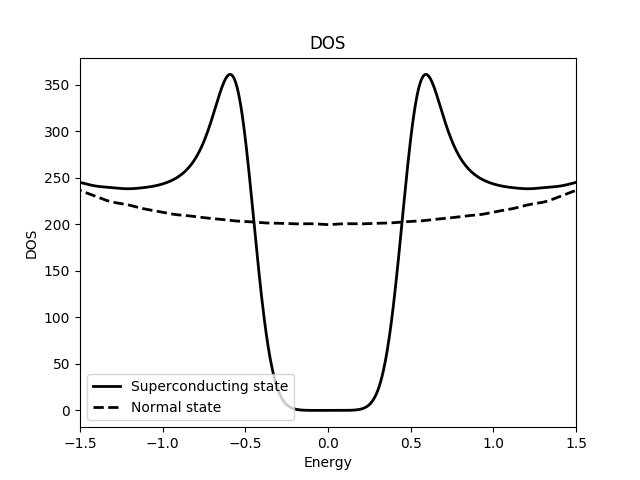
        if(n == 0){
            plotter.plot(
                dos,
                {
                    {"linestyle", "-"},
                    {"color", "black"},
                    {"label", "Superconducting state"}
                }
            );
        }
        else{
            plotter.plot(
                dos,
                {
                    {"linestyle", "--"},
                    {"color", "black"},
                    {"label", "Normal state"}
                }
            );
        }
    }
    plotter.save("figures/DOS.png");
}

Output